Theoretical background
Image Transformation
Overview of image transformations
- Translation
- Rigid or Euclidean (Rotation, translation)
- Similarity (Rotation, translation, scaling)
- Affine
- Projective
Consider a point $\mathbf{x}=(x,y)$ in the 2D space. Then we can define translation, rotation and scaling using the following equations which maps the points from $\mathbf{x} \to \mathbf{x}'$ where $\mathbf{x}' = (x',y)'$ is the new transformed coordinates.
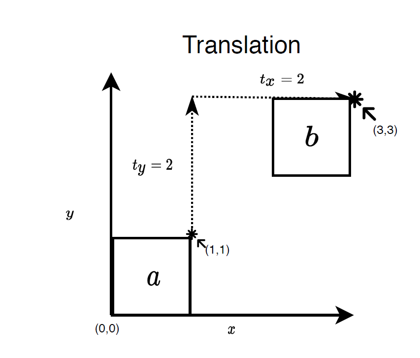
Translation
We can define the translation in $x$ and $y$ direction as below
- $x' = x + t_x$
- $y' = y + t_y$.
This can also be written in vector notation as follows:
- $\mathbf{x}' = \mathbf{x} + \mathbf{t}$ where $\mathbf{t} = (t_x, t_y)$
Rotation
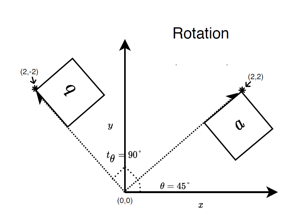
We can define the translation in $x$ and $y$ direction as below
- $x' = x cos\theta + y sin\theta$
- $y' = -x sin\theta + y cos\theta$
Scaling
We can define the translation in $x$ and $y$ direction as below
- $x' = sx$
- $y' = sy$.
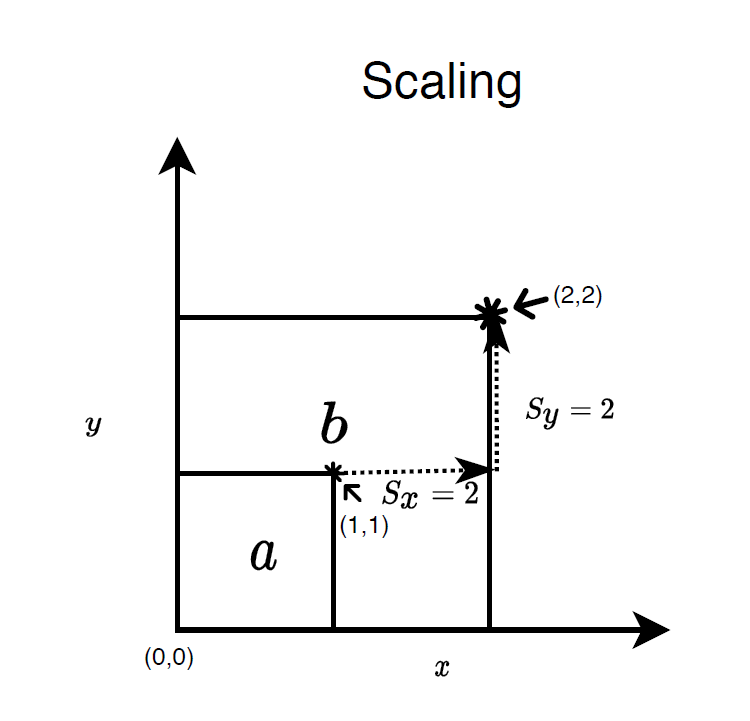
We can also chain the different transformations and compute the transformed coordinate using a single equation
$$x' = s (x \cos\theta + y \sin\theta ) + t_x$$ $$y' = s(-x \sin\theta + y \cos\theta) + t_y$$
Illustration of different transformation
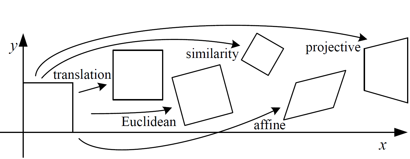
Image Source : Szeliski, Richard. Computer vision: algorithms and applications
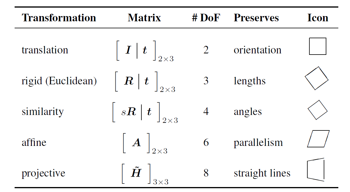
Image Source : Szeliski, Richard. Computer vision: algorithms and applications
For more details about image transformations, you can also check out the computer vision book by Richard Szeliski. A free pdf is available on the website.
Image interpolation
Let us consider an example image transformation. Initially we have an unit square with its left corner placed at the origin (0,0). Assume that we have image intensity values at the corners of the unit square at a = (0,0), b =(0,1), c = (1,1), d = (0,1).
We apply a small translation $\mathbf{t} = (0.5,0.5)$ to the square. As you can see in the image, now our left corner point is at $a' = (0.5,0.5)$. Since we don't have the value at this point we are forced to approximate the value from the information available to us. This is the main reason for implementing image interpolation function as image transformations can always lead to coordinates for which we don't have any value and we approximate the value using the neighbourhood information.
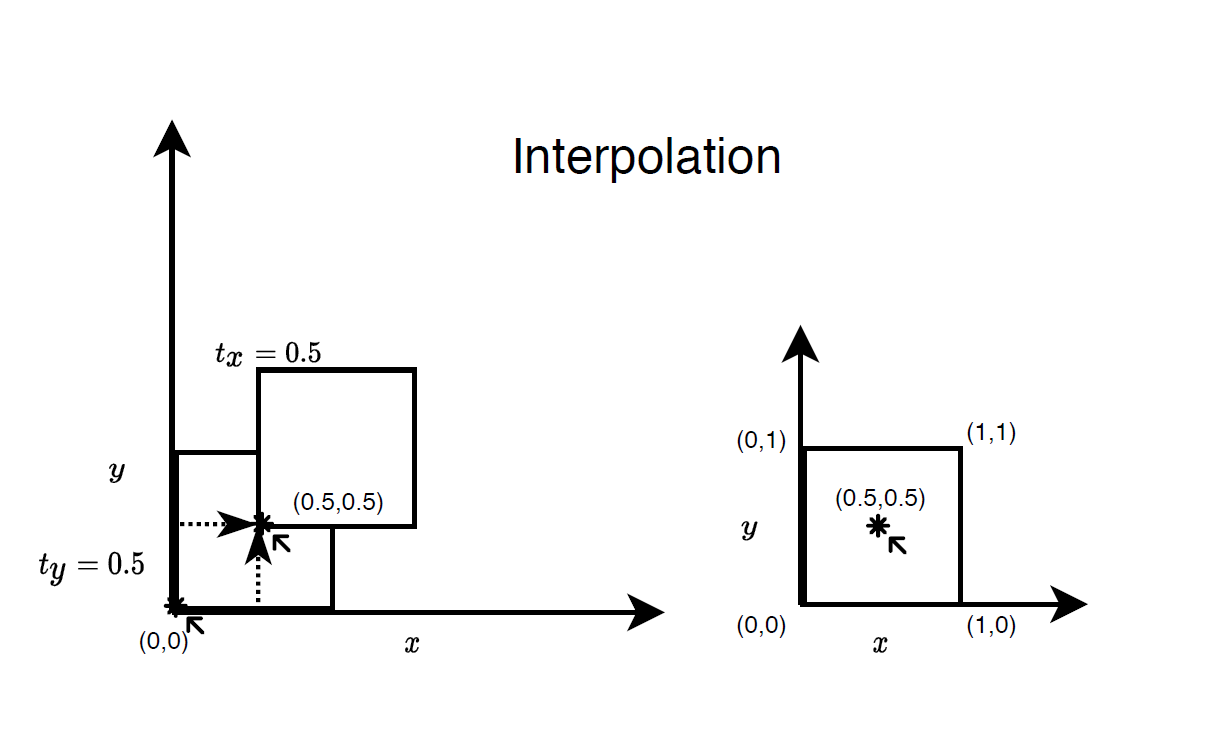
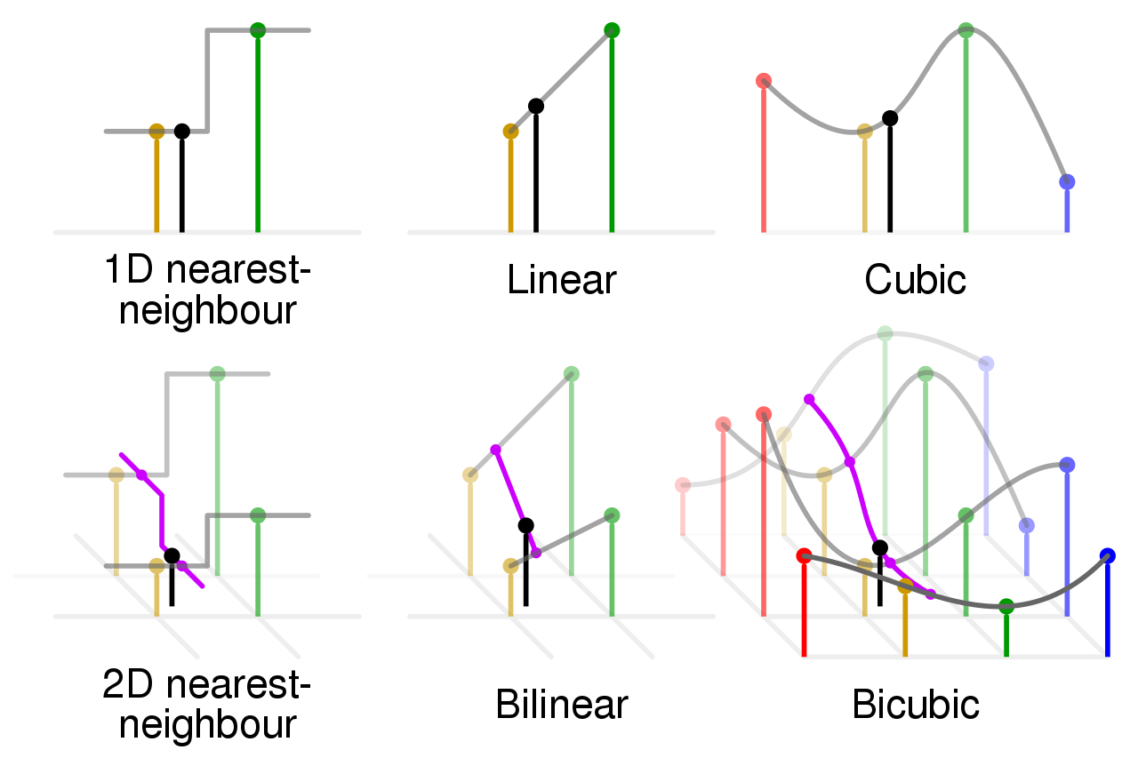
The way in which we use the neighbouring information governs the quality of the interpolated image. The different types of interpolation are as follows:
- Nearest neighbour
- Bilinear
- Bi-cubic
Illustration of different types of interpolation
The image below shows how the different types of interpolation works. The discrete points are the places where we know the function value and the lines connecting these points represents the interpolated function values.
We will implement only bilinear interpolation for our Image class. Lets dive a bit deeper into the bilinear interpolation and look at the how the values are interpolated using this method.
Bilinear interpolation
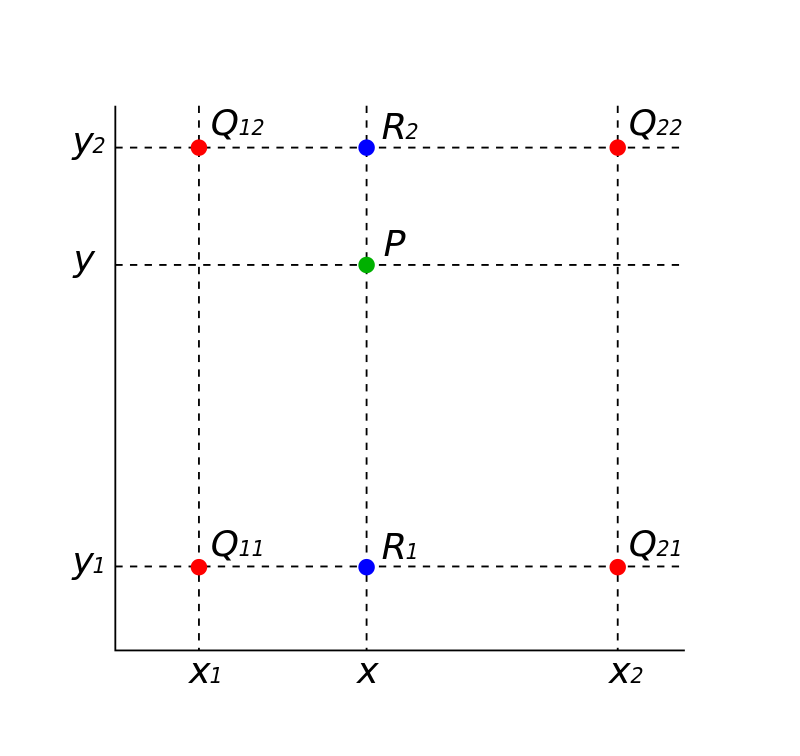
Consider the above image where the red dots ($Q_{ij}$) indicate the discrete points where we know the function value. We want to approximate the function value at point $P$.
Consider the points(red dots) in the above image:
$$Q_{11} = (x_1,y_1), Q_{21} = (x_2,y_1)$$
$$ Q_{12} = (x_1,y_2), Q_{22} = (x_2,y_2)$$
Assume that each of these points $Q_{ij}$ corresponds to an image pixel with intensity values.
Now we need to find the image intensity value at point $P= (x,y)$ which is in between the points $Q_{ij}$
Let us consider one coordinate at a time (i.e. $x_i$ or $y_i$) for interpolation. Here we intially interpolate along the $x$-axis. So now our aim is to find values at $P(x,y_i)$. (i.e. find intermediat values $R_i (x,y_i)$. We have two values of $y_i$ so we can find two intermediate values.)
We can obtain two such values by interpolating along $Q_{11}, Q_{21}$ and find out the intermediate value as $R_1$ and between $Q_{12}, Q_{22}$ and find out the intermediate value $R_2$.Look at the image of how we just interpolate along the line.
We can directly use the linear interpolation equation to find out the values of $f(R_1)$ and $f(R_2)$
$$ \frac{f(x) - f(x_1)}{x-x_1} = \frac{f(x_2) - f(x_1)}{x_2 - x_1} $$
Once we have the values at $R_1 = (x,y_1)$ and $R_2 = (x,y_2)$ we can again use the same linear interpolation formula along the $y$-axis and find the function value $f(P)$ at $P=(x,y)$.
This way we can interpolate(approximate) any values (x,y) if we know the neighbouring values. However when we actually implement the method we also need to find out the neighbouring values on our own as they are not provided.

